C Some Notes On Ellipses
The general equation of an ellipse centered at the origin can be written as \[ ax^2 + bxy + cy^2 = 1 \] where, as will be shown below, \(4ac - b^2 >0\). We will first calculate the area of the ellipse in terms of the above coefficients. Then we will proceed to write the equation of the ellipse in terms of a matrix where we can arrive at the correspondence between the matrix elements and the above coefficients. We will see that the area of the ellipse as found from analytic geometry will be equal to the determinant of an appropriate matrix describing the same ellipse.
C.1 Area of an Ellipse
From our general equation above, we solve for y as a function of x by re-writing as \[ c\;y^2 + bx\;y + (ax^2-1) = 0 \] and solving the quadratic equation for \(y\): \[ y_{\pm} = \frac{-bx \pm \sqrt{(b^2-4ac)x^2 + 4c} }{2c}. \] The two solutions correspond to the “upper” and “lower” portions of the ellipse, going from -\(x_0\) to +\(x_0\). The limits of \(x\) for this ellipse can be found by taking the derivative and noting that \(dy/dx \rightarrow \infty\) as \(\sqrt{(b^2-4ac)x^2+4c} \rightarrow 0\), yielding for these extrema at \(x = \pm x_0\) where \[ x_0 = \sqrt{\frac{4c}{4ac-b^2}} . \] We note that \(4ac>b^2\) for \(x_0\) to be real.
The area \({\cal A}\) of the ellipse can now be found by integrating the positive solution \(y_+\) and subtracting the integration of the negative solution \(y_-\) to obtain \[ {\cal A} = 2\int_{-x_0}^{x_0} \frac{\sqrt{4c-(4ac-b^2)x^2}}{2c}\; dx = \frac{4}{\sqrt{4ac-b^2}}\int_{-1}^{1} \sqrt{1-u^2} \;\; du \] where \(u \equiv x/x_0\). With the usual trigonometric substitution, this reduces to \[ {\cal A} = \frac{4}{\sqrt{4ac-b^2}}\int_{-\pi/2}^{\pi/2} \cos^2\theta\; d\theta \] or, \[ {\cal A} = \frac{2\pi}{\sqrt{4ac-b^2}}. \] Note that the maximum extent of the ellipse in the coordinate \(x\) can be also be identified as \[ \pm x_0 = \pm({\cal A}/\pi)\sqrt{c}, \] and, similarly, the maximum extent in the \(y\) direction is \[ \pm y_0 = \pm ({\cal A}/\pi)\sqrt{a}. \]
C.2 Equation of Ellipse – Matrix Notation
Let us now re-start our analysis by writing the equation of our ellipse in matrix notation. Let \(\vec{X}\) be the vector \[ \vec{X} = \left(\begin{array}{c} x \\ y \end{array}\right) \] and let \(A\) be a general \(2\times 2\) matrix, \[ A = \left(\begin{array}{cc} a_{11} & a_{12} \\ a_{21} & a_{22} \end{array}\right) . \] With \(\vec{X}^T\) being the transpose of \(\vec{X}\), then we can see that \[ \vec{X}^T A \vec{X} = \left( x ~~~ y \right) \left(\begin{array}{cc} a_{11} & a_{12} \\ a_{21} & a_{22} \end{array}\right) \left(\begin{array}{c} x \\ y \end{array}\right)= a_{11}\; x^2 + (a_{12} + a_{21})\; xy + a_{22}\; y^2 = 1 \] would be the equation of an ellipse. If we demand \(A\) be a symmetric matrix (\(a_{21} = a_{12}\)), then we would see the immediate correspondence to our original ellipse equation: \[ a_{11}\; x^2 + 2a_{12}\; xy + a_{22}\; y^2 \;\; = \;\; a\; x^2 + b\; xy + c\; y^2 = 1 \] and so \(a \leftrightarrow a_{11}\), \(b \leftrightarrow 2a_{12}\), and \(c \leftrightarrow a_{22}\). Using our previous result for the area of the ellipse, we find that \[ {\cal A} = \frac{2\pi}{\sqrt{4ac-b^2}} = \frac{2\pi}{\sqrt{4a_{11}a_{22}-4a_{12}^2}} = \frac{\pi}{\sqrt{\det A}} \] where \(\det A\) is the determinant of the matrix \(A\).
Thus, to recap, given a general equation of an ellipse centered at the origin \[ ax^2+bxy+cy^2 = 1 \] a symmetric matrix \(A\) can be formed, namely \[ A = \begin{pmatrix}a & b/2 \\ b/2 & c \end{pmatrix} \] such that the ellipse equation can be written as \[ \vec{X}^T A \vec{X} = 1. \] The area of the ellipse is then given by \[ {\cal A} = \frac{\pi}{\sqrt{\det A}}. \]
C.3 Particle Distributions and the Sigma Matrix
We wish to generate an appropriate matrix representation to describe our particle beam distributions and their area in phase space – the beam emittance. To visualize the situation, imagine a particle distribution in which each of our two variables \(x\) and \(y\) are distributed normally about the origin, but with a possible correlation as shown below:
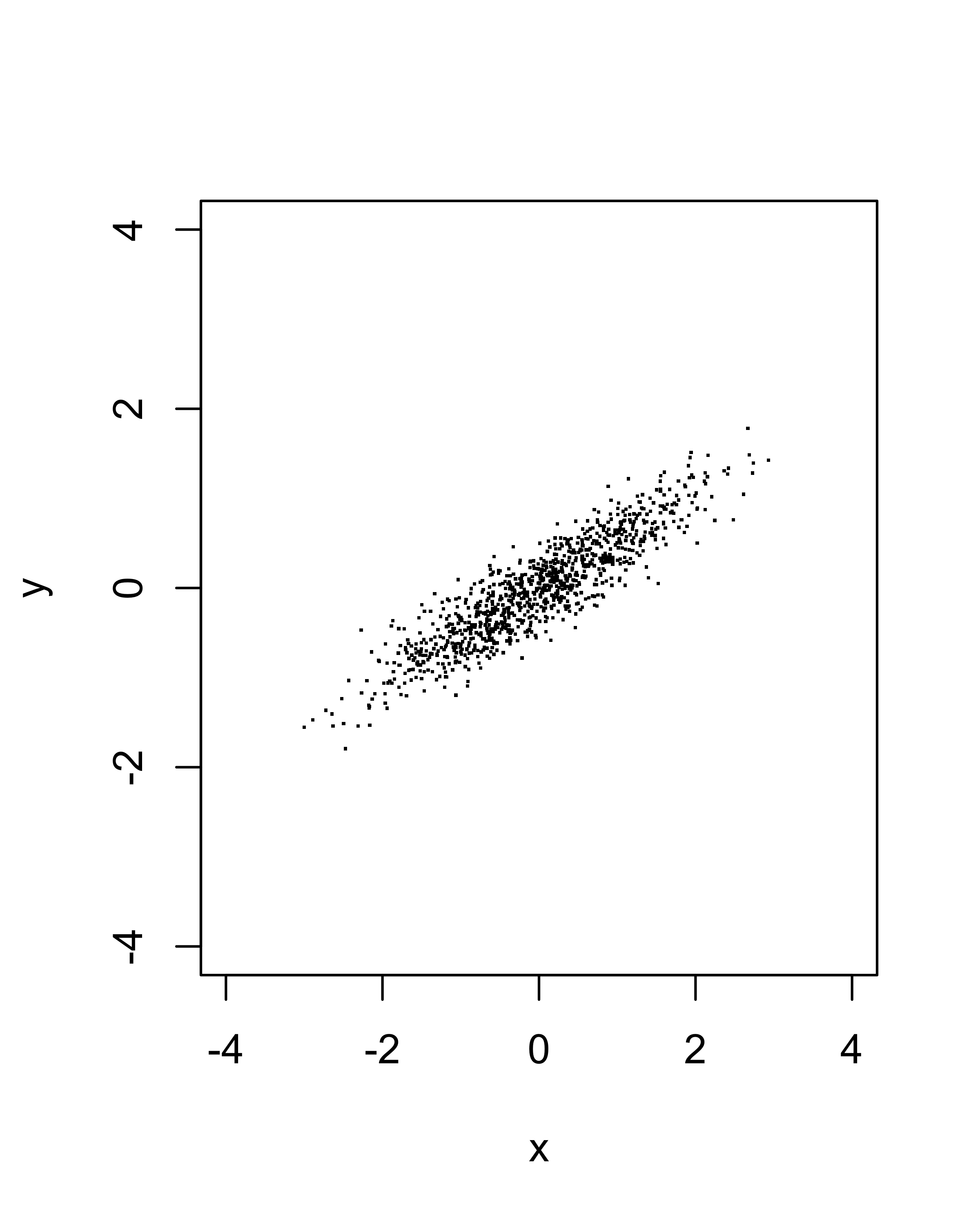
The image above certainly has an “elliptical” character to it, and it is easy to imagine drawing an ellipse that contains all, or a significant fraction, of the particles. We wish to formalize the development of such an ellipse that can be used to describe the general orientation and eccentricity of the distribution and to characterize its area.
We begin by creating a matrix \(\Sigma\) made by forming the product \(\vec{X}\vec{X}^T\) and taking the average values across the distribution of each of its elements: \[ \langle \vec{X}\vec{X}^T \rangle = \langle \left(\begin{array}{c} x \\ y \end{array}\right) ( x \;\;\; y)\rangle = \left(\begin{array}{cc} \langle x^2 \rangle & \langle xy \rangle \\ \langle xy \rangle & \langle y^2 \rangle \end{array}\right) = \left(\begin{array}{cc} \sigma_{11} & \sigma_{12} \\ \sigma_{12} & \sigma_{22} \end{array}\right) \equiv \Sigma \] where \(\langle f \rangle = \frac{1}{N} \sum_{i=1}^{N} f_i\). Note that this matrix \(\Sigma\) is automatically symmetric.
The inverse of \(\Sigma\) is \[ \Sigma^{-1} = \left(\begin{array}{cc} \sigma_{22} & -\sigma_{12} \\ -\sigma_{12} & \sigma_{11} \end{array}\right)\cdot \frac{1}{\det\Sigma}. \] If we use this inverse matrix to create an ellipse equation, \[ \vec{X}\Sigma^{-1}\vec{X}^T = 1 \] then this leads to the form: \[ \sigma_{22}\;x^2 - 2\sigma_{12}\;xy + \sigma_{11}\;y^2 = \det\Sigma . \] Noting that \[ \det \Sigma = \frac{1}{\det\Sigma^{-1}} \] and remembering that we used the matrix \(\Sigma^{-1}\) to form our ellipse equation, then \[ \sigma_{22}\;x^2 - 2\sigma_{12}\;xy + \sigma_{11}\;y^2 = ({\cal A}/\pi)^2. \]
C.4 Courant-Snyder Parameters and Emittance
We now use the above treatment to describe a particle beam distribution in phase space where \(x\) is the distance from the design trajectory along the longitudinal coordinate \(s\), and \(x'\) is the slope of the trajectory, \(x'=dx/ds\).
As shown earlier, the maximum extent of the ellipse in each coordinate is proportional to the square root of the area of the ellipse. Let \(\epsilon\) be the area of our relevant phase space distribution. Identifying \(y = x'\) in our treatment above, we now define new variables that relate the \(\sigma\) elements to the ellipse area: \[\begin{eqnarray*} \alpha &\equiv& -\sigma_{12}/(\epsilon/\pi) = -\langle xx'\rangle/(\epsilon/\pi)\\ \beta &\equiv& ~~ \sigma_{11}/(\epsilon/\pi) = ~~ \langle x^2\rangle/(\epsilon/\pi)\\ \gamma &\equiv& ~~ \sigma_{22}/(\epsilon/\pi) = ~~ \langle x'^2\rangle/(\epsilon/\pi) \end{eqnarray*}\]The Sigma Matrix is now \[ \Sigma = \begin{pmatrix} \langle x^2\rangle & \langle xx'\rangle\\ \langle xx'\rangle & \langle x'^2\rangle \end{pmatrix} = \begin{pmatrix} \beta\epsilon & -\alpha\epsilon\\ -\alpha\epsilon & \gamma\epsilon \end{pmatrix} \] and we find that the equation of our phase space ellipse can be written as \[ \gamma\;x^2 + 2\alpha\;xx' + \beta\;x'^2 = \epsilon/\pi. \] The parameters \(\alpha\), \(\beta\), and \(\gamma\) are referred to as the Courant-Snyder parameters.4 They determine the orientation and eccentricity of an ellipse that mimics the orientation and shape of the particle distribution, while the size of the ellipse is governed by \(\epsilon\). In accelerator and beam physics language, the area in phase space, \(\epsilon\), containing the particles is called the emittance.
From the way we introduced the Courant-Snyder variables above, we have chosen a particular ellipse: the one whose maximum extent in \(x\), for example, is \[ x_0 = (\epsilon/\pi)\sqrt{c} = (\epsilon/\pi)\sqrt{\sigma_{11}/(\epsilon/\pi)^2} = \sqrt{\sigma_{11}} = \sqrt{\langle x^2\rangle} = x_{rms}, \] and likewise \(x'_0 = x'_{rms}\). The emittance defined by this ellipse is often called the “rms emittance” and it is easy to verify that the rms emittance is given by \[ \epsilon = \pi \sqrt{\langle x^2\rangle\langle x'^2\rangle - \langle xx'\rangle^2 }. \] Note, too, that the product \[ \beta\gamma-\alpha^2 = [\sigma_{11}/(\epsilon/\pi)]\;[\sigma_{22}/(\epsilon/\pi)] - [\sigma_{12}/(\epsilon/\pi)]^2 = \det\Sigma/(\epsilon/\pi)^2 = 1. \] This shows that the three Courant-Snyder parameters are not independent. The third parameter is typically defined in terms of the other two: \[ \gamma = \frac{1+\alpha^2}{\beta}. \]
C.5 A Numerical Example
In our figure shown previously, we have used 1000 particles where the rms values of the two coordinates are \(x_{rms}\) = 1.018 and \(y_{rms}\) = 0.574; the coordinates are “correlated” with \(\langle xy \rangle\) = 0.53, and the determinant \(\det\Sigma\) has a value of 0.061.
Let us compute the values of the Courant-Snyder parameters and the rms area (emittance) of the distribution:
s11 = mean(x*x)
s22 = mean(y*y)
s12 = mean(x*y)
eps.pi = sqrt(s11*s22-s12^2)
alf  = -s12/eps.pi
bet  =  s11/eps.pi
gam  =  s22/eps.pi
## [1] Assuming x in mm, and y = x' = dx/ds in mr, then## [1] rms emittance = 0.247 pi mm-mr## [1] alpha = -2.14 , beta = 4.19 m, gamma = 1.33 /m.Now, we replot our particle distibution and draw ellipses with areas \(\epsilon\) and \(6\epsilon\) using the above-found Courant-Snyder parameters:
x0 = sqrt(s11)
ellPlot = function(n,color){
   curve( ( sqrt(bet*n*eps.pi-x*x)-alf*x)/bet, xlim=c(-1,1)*sqrt(n)*x0,
      col=color, add=TRUE,lty=2,lw=2,n=500)
   curve( (-sqrt(bet*n*eps.pi-x*x)-alf*x)/bet, xlim=c(-1,1)*sqrt(n)*x0,
      col=color, add=TRUE,lty=2,lw=2,n=500)
}
plot(x,y, xlim=c(-1,1)*lim, ylim=c(-1,1)*lim, pch=".",
   main="rms (blue), 95% (red) emittances")
ellPlot(1,"blue")
ellPlot(6,"red")
text(-3,3,paste(Num," particles"))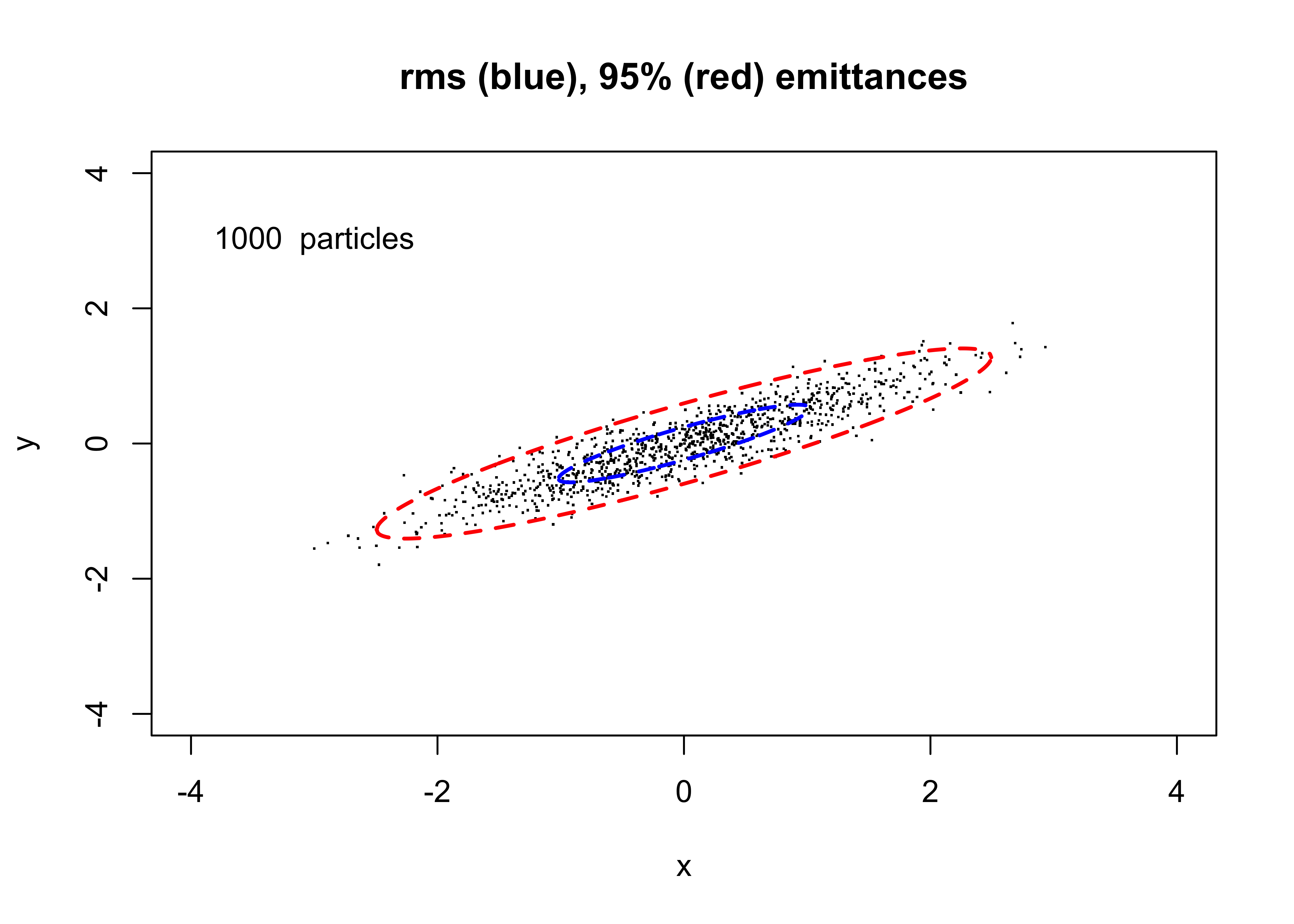
For Gaussian distributions, the curve of area \(\epsilon_{rms}\) should contain about 39% of the particles, while the curve of area \(6\epsilon_{rms}\) should contain roughly 95% of the particles.
C.6 Propagation of Courant-Snyder Parameters
For the case of our particle beam being propagated through magnetic bending and focusing elements – assuming fields that depend at most linearly with transverse position – the transverse position and slope of the particle trajectory is governed by a linear transformation \(M\) in going from point “1” to point “2”: \[ \vec{X_2} = M\vec{X_1}. \] In our energy-conserving Hamiltonian system, \(M\) will have unit determinant.
If we form the \(\Sigma\) matrix at point 2, we can see how the \(\Sigma\) matrix transforms between point 1 and point 2: \[ \Sigma_2 = \langle \vec{X_2}\vec{X_2}^T \rangle = \langle M\vec{X_1} (M\vec{X_1})^T \rangle = \langle M\vec{X_1} \vec{X_1}^TM^T \rangle = M\Sigma_1 M^T. \] Since \(\det M = 1\), then from the above equation we see that \(\det\Sigma_2 = \det\Sigma_1\) – the phase space emittance is an invariant during the beam propagation through the focusing system. If we define \(K\) as the matrix of Courant-Snyder parameters formed by dividing \(\Sigma\) by the rms emittance, \[ K = \frac{1}{\epsilon} \; \Sigma = \left( \begin{array}{cc} \beta & -\alpha \\ -\alpha & \gamma \end{array} \right), \] then \(K\) transforms according to \[ K_2 = M K_1 M^T. \] Hence, irregardless of the particle beam emittance, the eccentricity and orientation of the rms phase space ellipse will evolve along the beam line according to the above equation. If we know the values of the ellipse parameters at one point along our beam line, and we know the transport matrix from there to a downstream point, then we can find the values of the ellipse parameters at the new point accordingly.
C.7 Extension to Multiple Dimensions
In most accelerator and beam transport systems, particularly those with high magnetic rigidity, systems of dipole and quadrupole fields are used and extensive attempts are made to keep the motion in one transverse degree of freedom (\(x\)) independent from the other (\(y\)). For such a system, one can analyze the motion in \(x\) using \(2\times 2\) matrices describing trajectory development through each independent element and simultaneously use appropriate \(2\times 2\) matrices to describe motion in \(y\) through the same elements. In such cases, independent Courant-Snyder parameters for each plane can be used and “transported” through the magnetic system to develop beam envelopes and optical functions.
The Courant-Snyder description – utilizing amplitude functions and phase advance – breaks down when the motion in the two degrees of freedom are coupled. For uncoupled motion, a general \(4\times 4\) matrix operating on the vector \[ \vec{X} = \left( \begin{array}{c} x \\ x' \\ y \\ y' \end{array}\right) \] would have the block diagonal form \[ M = \left( \begin{array}{cccc} m_{11} & m_{12} & 0 & 0 \\ m_{21} & m_{22} & 0 & 0 \\ 0 & 0 & m_{33} & m_{34} \\ 0 & 0 & m_{43} & m_{44} \end{array}\right) \] and each block could be used to independently operate on the vectors \(\vec{X}\) and \(\vec{Y}\), for example, leading to Courant Snyder parameters \(\beta_x\), \(\beta_y\), and so on, for the two phase space ellipses for the two degrees of freedom.
But in the case that the particle motion is coupled between the four phase space variables – such as in the case of transport through a solenoidal magnetic field, or where ideal quadrupole fields are rotated about the longitudinal beam axis – then the traditional Courant-Snyder description is no longer valid.5 However, our matrix treatment using a “\(\Sigma\)” matrix is indeed still valid. The determinant of a \(4\times 4\) \(\Sigma\) matrix will still be an invariant of the motion, and the matrix elements will still propagate according to \(\Sigma_2 = M\Sigma_1 M^T\), which includes the development of all the correlations among the various coordinates. Indeed one can extend the treatment to \(6\times 6\) matrices that includes linearized motion in longitudinal coordinates as well (energy and time of flight, momentum and path length deviations, corrlations between position and momentum (dispersion), etc.).
See E.D. Courant and H.S. Snyder, Theory of the Alternating Gradient Synchrotron, Ann. Phys. 3, 1 (1958).↩
For more complete treatment of coupled degrees of freedom, see for example, D.A. Edwards and L.C. Teng, “Parameterization of Linear Coupled Motion in Periodic Systems”, IEEE Trans. Nucl. Sci. NS-20, No. 3 (1973); H. Mais and G. Ripken, “Theory of Coupled Synchro-Betatron Oscilliations I”, DESY M-82-17 (1982); I. Borchardt, E. Karantzoulis, H. Mais, G. Ripken, “Calculation of Beam Envelopes in Storage Rings and Transport Systems in the Presence of Transverse Space Charge Effects and Coupling”, DESY 87-161 (1987); and V.A. Lebedev and S.A. Bogacz, “Betatron Motion with Coupling of Horizontal and Vertical Degrees of Freedom”, Fermilab-Pub-10-383-AD (2012).↩